Introduction to the t-statistic

Z-tests vs. t-tests

Z-tests compare the means between a population and a sample and require information that is usually unavailable about populations, namely the variance/standard deviation. Single sample t-tests compare the population mean to a sample mean, but only require one variance/standard deviation, and that’s from the sample. This is where estimated standard error comes in. It’s used as an estimate of the real standard error, σM, when the value of σ is unknown. It is computed using the sample variance or sample standard deviation and provides an estimate of the standard distance between a sample mean, M, and the population mean, μ, (or rather, the mean of sample means). It’s an “error” because it’s the distance between what the sample mean is and what it would ideally be since we would rather have the population standard deviation. The formula for estimated standard error is s/√n.

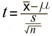
The formula for the t-test itself is:   with the bottom portion referring to the estimated standard error. You may see this written as sM instead.

Degrees of Freedom

Degrees of freedom describe the number of scores in a sample that are independent and free to vary. Because the sample mean places a restriction on the value of one score in the sample, there are degrees of freedom for a sample with n scores. For a single sample t-test, the degrees of freedom are calculated using the following formula: df = n-1.

Shape of a t-distribution

One general rule of t-distribution is that it’s always slightly flatter than it’s corresponding normal distribution. This is because t-statistics are always working from a sample size, which is relatively small, rather than a population, which are generally large.

There are some factors which also influence the shape of each individual t-distribution:

• The degrees of freedom: The greater n is, and subsequently df, the more like a normal distribution the t-distribution will begin to look (this also follows the 30 rule)
• The sample variance: The bottom half of the equation deals with the estimated standard error, which changes when the standard deviation changes. Because the ESE is dependent on the sample variance, each sample can create a different ESE

Hypothesis Testing with a Single Sample t-test

The written null and alternative hypotheses for a single sample t-test are as follows:

H0 : μ = population mean

H1 : μ ≠ population mean

The stops for a single sample t-test are as follows: 

1. State the hypotheses and select an alpha level
2. Locate the critical region
3. Calculate the test statistic
4. Make a decision regarding the null hypothesis

The following are some assumptions one makes when doing a single sample t-test:

• The values in the sample must consist of independent observations.
• The population that is sampled must be normal.

Effect Size for Single Sample t-tests

Effect size for a single sample t-test is calculated using Cohen’s d. The formula for this is the mean difference over the standard deviation, or (M – μ) / s. Effect size is important because it’s a way of quantifying the difference between two groups, rather than just saying that there is a significant difference. Essentially, it’s also important to know how much of a difference there is, not just the likelihood that the group differences you’re seeing are a fluke because the null hypothesis is actually true. This can also be important for practical significance. If your treatment is statistically significant, but has a small effect size, is it worth using this treatment on clients?

For Cohen’s d, 0.2 would be considered a small effect size, 0.5 is medium, and 0.8 is large. Some people will mix words together like “small to medium effect size” but some professors will want you to just pick a side. 

Confidence Intervals

Confidence intervals are a range of values which is likely to encompass the true value you’re looking for. More specifically, it’s a range we create using a sample that we can say with X% confidence that the population mean falls within that range. Confidence intervals are constructed at a confidence level, such as 95%, selected by the user. It means that if the same population is sampled on numerous occasions and interval estimates are made on each occasion, the resulting intervals would bracket the true population parameter in approximately 95% of the cases. Confidence intervals and any kind of interval estimation are used in the same situations that you would use hypothesis testing. There is an estimation procedure for every kind of hypothesis test.