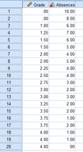
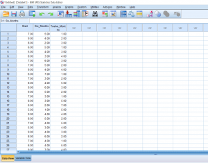
A correlation requires at least 2 continuous variables. We need to first define our variables in Variable View. In this case, we’re looking at how number of absences relates to grade point average.

Next, we type in our data points in Data View.

A correlation requires at least 2 continuous variables. We need to first define our variables in Variable View. In this case, we’re looking at how number of absences relates to grade point average.
Next, we type in our data points in Data View.
A regression can be seen as a kind of extension of a correlation. When doing a regression, you find a lot of the same outputs, like Pearson’s r and r-squared. The difference is that the point of a regression is to also construct a model (usually linear) that will help us predict values using a line of best fit. In the case of this example, we will be looking at average hours of sleep students get and comparing it to their GPA. A regression will also give us a model (y=mx+b) that would allow us to predict the GPA of a hypothetical student if we knew the average amount of sleep they get a night.
First, we need to create our variables in Variable View.
Then, we need to input our data into Data View. You can’t see it in this photo, but I have 25 participants total. Continue reading
Many statistical tests run on the assumption that the data with which you are working is normally distributed, so it’s important to check. There are several different ways to go about this,. This post will explain a few different methods for testing normalcy as well as provide some instructions about how to run these tests in Excel.
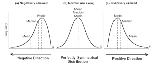
An important rule to note about distribution is that in a normal distribution, the mean, median, and mode are approximately equal. What it looks like visually is that the mean, median, and mode are all sitting at the top of the hump of the bell curve. When a distribution is skewed, these values become different. The mode will always sit around the hump of a distribution (because this is where most of the values have accumulated). The mean is the measure of central tendency most affected by extreme variables and outliers, so it will follow the longest tail. The median, in this case, will always fall somewhere between the median and the mode. Put another way, if the distribution is positively skewed, the mean will be the greatest value, the median will be the second greatest value, and the mode will be the smallest value. If the distribution is negatively skewed, the mean will be the smallest value, the median will be the second smallest value, and the mode will be the greatest value. So when you’re looking at a data set, you may be able to get an idea of the skew of the distribution by comparing the mean and the median.
Reading graphs of two-way ANOVAs is often a little frustrating at first for students who are new to reading them. The goal of this post is to hopefully make the process more straight-forward.
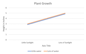
If you’re not sure already what a main effect or interaction is, I would suggest heading over to another post about two-way ANOVAs first. The purpose of one of these graphs is to help the reader visualize the results of the test when reading the results can sometimes be overwhelming, especially if the researchers are working with several different levels in each independent variable. The first trick to remember is that when looking for a significant main effect in the variable on the X-axis, we want the mean distance between the two points above one condition to be different from the mean distance between the two points of another condition. A clear example of this is below. The middle point between the orange line and blue line above “Little Sunlight” is around 2.8, while the middle point between the orange line and blue line above “Lots of Sunlight” is about 4.8. Given the context, we would say that there is a main effect for sunlight in which plant growth increases as levels of sunlight increase.
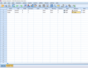
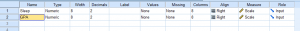
Just like an independent samples t-test, an Independent measures one-way ANOVA uses independent subjects for each level/condition within an independent variable. In this example, we’re growing plants. In Variable View, I’ve made the independent variable Condition (in this case the amount of water I’ll be giving to the plants) and the dependent variable Height.
This post will be about finding a difference in means when it comes to repeated measures in research designs with a factor with more than 2 levels. Just like with the Repeated Measures t-test, we’ll be lining our levels up in columns. For this example, we’ll pretend that we’ve collected data on self-reported depression. Participants were asked to rate on a scale from 1-9 how severe they felt their depression is. They were then given medication to take which is known to reduce depressive symptoms. Participants were asked again after 6 months how high they rated their depression. They were asked one last time at the end of 12 months.
In this section, we’ll be talking about how to properly conduct a repeated measures t-test on SPSS. Before, when we were working on independent t-tests, we needed to create a list of numbers which represented group categories so that the corresponding continuous data was grouped properly. In this kind of t-test though, each “Variable” actually becomes a level. In this case of this example, we’re looking at the data from a before and after. The “Before” consists of the number of alcoholic drinks 30 college students are consuming a week. The “After” consists of the number of alcoholic drinks the same college students were drinking after having taken a Wellness class which focused on the effects of drug and alcohol on the mind and body. If you’re confused as to how this differs from an independent samples t-test, I suggest looking at the Independent Samples t-test and Repeated Measures t-test posts. 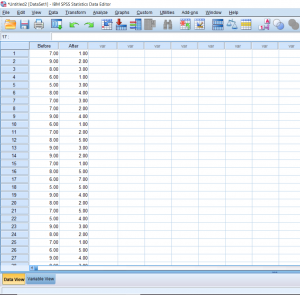 Continue reading
In this section, we’ll be talking about finding the probability of a sample proportion. You may remember that a sampling distribution is a distribution not of scores, but all possible sample outcomes which can be drawn given that we’re working with a specific n. In this case, the following equations can help us figure out, based on a population proportion, how likely it is that we’ll draw a sample that has a chosen proportion. A question which would require these equations may sound like the following:
“A nation-wide survey was conducted about the perception of a brand. People were asked whether they liked the brand or disliked the brand and the results showed that 65% of people liked the brand. If we were to draw a random sample of 200 people, what is the probability that 80% of people within that sample will say they like the brand?”
The population proportion, denoted as ?, is the proportion of items in the entire population with the particular characteristic that we’re interested in investigating. The sample proportion, denoted by p, is the proportion of items in the sample with the characteristic that we’re interested in investigating. The sample proportion, which by definition is a statistic, is used to estimate the population proportion, which by definition is a parameter. Continue reading
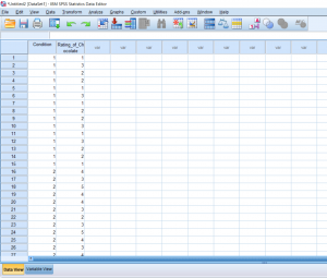
So far we’ve talked about creating independent variables, but what about levels? This may seem strange at first, but levels of a condition need to be spelled out by numbers. Usually, I just assign condition 1 a 1 and condition 2 a 2. You can see in the picture below how this looks. You can’t see this, but there are 30 individuals in total, half in condition 1, and half in condition 2.
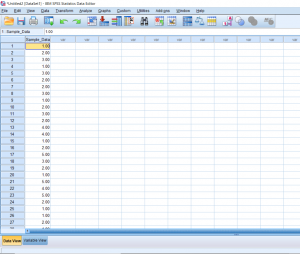
With a one-sample t-test, we only need to worry about working with one sample. When starting, you should already know the population mean you’ll be comparing the sample to. So in this first picture, we have one column of data lined up and ready to go.