Basics of Variability

Variability is often a difficult topic for newcomers to statistics to grasp. Essentially it is the spread of the scores in a frequency distribution. If you have a bell curve which is pretty flat, you would say that it has high variability. If you have a bell curve which is pointy, you would say that it has low variability. Variability is really a quantitative measure of the differences between scores and describes the degree to which the score are spread out or clustered together. The purpose of measuring variability is to be able to describe the distribution and measure how well an individual score represents the distribution.

There are three main types of variability:

• Range: The distance between the lowest and the highest score in a distribution. Can be described as one number or represented by writing out the lowest and highest number together (ex. values 4-10). Calculated by subtracting the highest score from the lowest score. If you’re working with continuous variables, it’s the upper real limit for Xmax minus the lower real limit for Xmin.
• Standard deviation: The average distance between the scores in a data set and the mean. Here’s a video to help you conceptualize this. This value is also the square root of the variance.
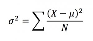
• Variance: Measures the average squared distance from the mean. This number is good for some calculations, but generally we want the standard deviation to determine how spread out a distribution is. Calculated with this equation:

Sample Variance and Degrees of Freedom

Sample variance is just the variance that needs to be calculated as a substitute sometimes when the population variance is unavailable (this will be talked about more later). Here’s a video explaining this more. The degrees of freedom determine the number of scores in the sample that are independent and free to vary. This is important because in a sample, all the data points are allowed to be whatever score, but the last score needs to be such that the mean we calculated stays that mean. So if we have 3 scores in a set, and we know the mean is 5, the first two scores can be any numbers, in this case it’s 9 and 2. Because we calculated that the mean is 5, the last number has to be 4 to add up to 15 and divide by 3 to get 5. The last score is dependent on the other scores. Al this means practically is that the equation of sample variance differs from population variance in that the denominator is n-1. So n-1 literally means that all the scores except the “last” one are allowed to be whatever they want. Here’s a video with some more explanation.

Biased vs. Unbiased

An unbiased estimate of a population parameter is when the average value of a statistic is equal to the parameter and the average value uses all possible samples of a particular size n. A biased estimate of a population parameter systematically overestimates or underestimates the population parameter. In this case, we know that sample variability tends to underestimate the variability of the corresponding population. We correct this by using degrees of freedom and we account for this when we use standard error.

Inferring Patterns in Data

Variability in the data influences how easy it is to see patterns. High variability obscures patterns in comparing two sets of data that would be visible in low variability samples. It can’t tell you if there’s a significant difference between groups, though. You have to run an analysis of variance or t-test to determine that.