Repeated Measures One-way ANOVA

Just like when we talked about independent samples t-tests and repeated measures t-tests, ANOVAs can have the same distinction. Independent one-way ANOVAs use samples which are in no way related to each other; each sample is completely random, uses different individuals, and those individuals are not paired in any meaningful way. In a repeated measures one-way ANOVA, individuals can be in multiple treatment conditions, be paired with other individuals based on important characteristics, or simply matched based on a relationship to one another (twins, siblings, couples, etc.). What’s important to remember that in a repeated measures one-way ANOVA, we are still given the opportunity to work with multiple levels, not just two like with a t-test.

Advantages:

• Individual differences among participants do not influence outcomes or influence them very little because everyone is either paired up on important participant characteristics or they are the same person in multiple conditions.
• A smaller number of subjects needed to test all the treatments.
• Ability to assess an effect over time.

Disadvantages:

• Increases the likelihood that outside factors that change over time may be responsible for changes in the participants’ scores.
• Participation in the first treatment could affect scores in the second treatment (practice, fatigue, etc.).

Hypothesis Testing with Repeated Measures One-Way ANOVA

The null and alternative hypotheses for a repeated measures ANOVA are as follows:

H0 : µ1 = µ2 = µ3

H1: µ1 ≠ µ2 ≠ µ3

Assumptions of repeated measures one-way ANOVAs are as follows:

• The observations within each treatment condition must be independent.
• The population distribution within each treatment must be normal
• The variances of the population distribution for each treatment should be equivalent

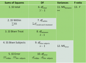
The steps to calculating a repeated measures one-way ANOVA are explained in this chart.

Here is a link to a video you may find useful. Please remember that different disciplines use different versions of the same equations; don’t let this intimidate you. Just use what you have been given by your book or professor.

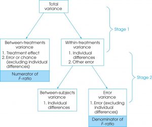
There is a conceptual meaning underlying the process of calculating this. There are more sums of squares to consider because we’re doing our best to separate within differences from between differences but also distinguishing which within differences are due to individual differences between the subjects and what error can’t be accounted for by individual differences. So instead of basing an F-ratio on the balance of between treatment differences and any error that could ever take place, we reduce the error being used to calculate whether there’s a significant difference by getting rid of the kind of error we can measure with a repeated measures design: participant differences. See the graphic below for a visual representation of this concept. 

Effect Size

Effect size, in this case, is calculated once again using partial eta squared:

η2 = SSBetweenTreatments / SStotal  – SSBetweenSubjects

Be careful not to accidentally plug in the wrong value, as these names all sound similar to one another. The numerator should be the between treatments sum of squares gotten in the first step of the calculation. The denominator is the total sum of squares minus the between-subjects sum of squares found in the second round of calculations.

Post Hoc Tests

Like we mentioned in the previous post, post hoc tests are tests run to determine which groups are significantly different from one another after determining through the ANOVA that there’s a significant difference somewhere. Is the significant difference between A and B, B and C, C and A, or all three? For repeated measures one-way ANOVAs, Tukey’s HSD and Scheffe can be used, just substitute SSerror and dferror in the formulas. These formulas can be found on the statistics formula glossary post.