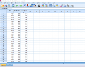
This post will be about finding a difference in means when it comes to repeated measures in research designs with a factor with more than 2 levels. Just like with the Repeated Measures t-test, we’ll be lining our levels up in columns. For this example, we’ll pretend that we’ve collected data on self-reported depression. Participants were asked to rate on a scale from 1-9 how severe they felt their depression is. They were then given medication to take which is known to reduce depressive symptoms. Participants were asked again after 6 months how high they rated their depression. They were asked one last time at the end of 12 months.

I went ahead and named the levels in the Variable view.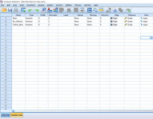

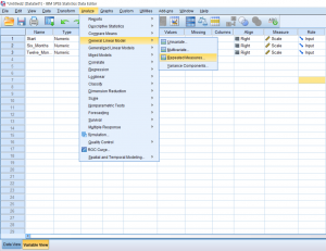
To run the actual test, simply go up to Analyze, scroll over General Linear Model, and click Repeated Measures.

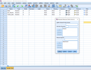
A pop-up will appear. In the first box, create the name of your factor. In this case, I’ve named it time, because we’re doing comparisons across time. In the second box, I typed in 3 because we have 3 levels and then I pressed Add. In the third box, I named our dependent variable and clicked Add. Next, we need to Define our factors…

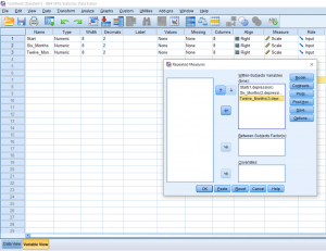
Another pop up will appear. Move the levels over into the top, right box. I prefer doing this in chronological order from top to bottom. Then, click Options.

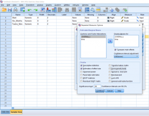
I would recommend getting means for everything, so move OVERALL and time over to the box on the right. I also recommend clicking the Descriptive Statistics and Estimate of Effect Size boxes. Finally, click the Compare Means checkbox; it’s located under the big, white box on the right. Click all the Continues and OK’s that follow.

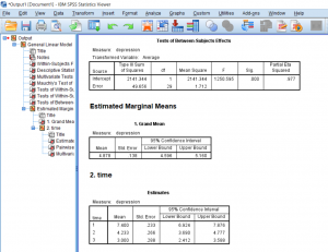
We can see from the means that the average for Start is greater than at 6 months is greater than at 12 months. This is important to know, but this does not prove significance.

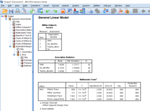
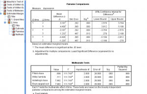
Go to the Tests of Within-Subjects Effects box and find “time” on the left, scroll over to Greenhouse-Geisser, and then scroll all the way to F and significance. We have a huge F score of 68.5 and a significance which is less than 0.05 and so we can say that somewhere there is a significant difference in the groups. If you need to report the effect size, you can find it under Partial Eta Squared.

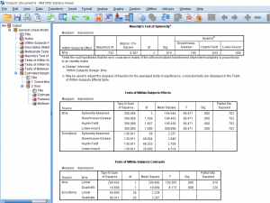
This last box shows us the post-hoc under Pairwise Comparison. As you can see, all the comparisons are significantly different with a significance less than 0.05. This means that we can say that there was a significant difference in times since treatment began with participants expressing the most depression before the treatment started, less depression 6 months after the treatment started, and the least depression after 12 months of treatment.