Category Archives: PUAD 628

Statistics: Independent One-Way ANOVA

Independent One-way ANOVA

An ANOVA (ANalysis Of VAriance) is a test that is run either to compare multiple independent variables with two or more levels each, or one independent variable with more than 2 levels. You can technically also run an ANOVA in the same cases you would run a t-test and come up with the same results, but this isn’t common practice, as t-tests are easier to compute by hand.

For the purposes of this post, a One-way ANOVA is a test which compares the means of multiple samples (more than 2) which are connected by the same independent variable. An example of this might be comparing the growth of plans who receive no water (Group 1) a little water (Group 2), a moderate amount of water (Group 3), and a lot of water (Group 4).

factor is another name for an independent variable. As mentioned earlier, ANOVAs can sometimes have more than one factor, but for now we’re only working with one, just like we have before. A level is a group within that independent variable. Using the example from before, the groups in which the plants are put in are the levels (no water, little water, some water, a lot of water) and the independent variable itself is just water amount. Continue reading

Statistics: Repeated Measures t-test

Repeated Measures T-Test

A repeated measures or paired samples design is all about minimizing confounding variables like participant characteristics by either using the same person in multiple levels of a factor or pairing participants up in each group based on similar characteristics or relationship and then having them take part in different treatments. Matched subjects is another word used to describe this kind of test and it is used specifically to refer to designs in which different people are matched up by their characteristics. Participants are often matched by age, gender, race, socioeconomic status, or other demographic features, but can also be matched up on other characteristics the researchers might consider possible confounds. Twin studies are a good example of this kind of design; one twin has to be matched up with the other – they can’t be matched to someone else’s twin.

To reiterate the differences between a repeated measures t-test and the other kinds of tests you may have learned up to this point, a single sample t-test revolves around drawing conclusions about a treated population based on a sample mean and an untreated population mean (no standard deviation). An independent sample t-tests are all about comparing the means of two samples (usually a control group/untreated group and a treated group) to draw inferences about how there might be differences between those two groups in the broader population. Different, randomly assigned participants are used in each group. Related samples t-tests are like independent sample t-tests except they use the same person for multiple test groups or they match people based on their characteristics or relationships to cut down on extraneous variables which may interfere with the data. Continue reading

Statistics: Independent t-tests

Independent t-test

In our last post, we talked about single sample t-tests, which is a way of comparing the mean of a population with the mean of a sample to look for a difference. With two-sample t-tests, we are now trying to find a difference between two different sample means. More specifically, independent t-tests involve comparing the means of two samples which are distinctly different from one another in regards to the individuals within each sample. For example, a group of pet owners vs. a group of folks who don’t own pets. These two groups are completely independent of one another. This distinction will be important in a later post.

A more technical explanation of the difference between a single sample and two-sample is that a single sample t-test revolves around drawing conclusions about a treated population based on a sample mean and an untreated population mean (no standard deviation). An independent sample t-tests are all about comparing the means of two samples (usually a control group/untreated group and a treated group) to draw inferences about how there might be differences between those two groups in the broader population

There are some distinct advantages and disadvantages to this approach when compared to other approaches. To avoid confusion, we won’t describe the other approaches here but will just mark the advantages and disadvantages of this one here for your consideration: Continue reading

Statistics: Introduction to the t-statistic

Introduction to the t-statistic

Z-tests vs. t-tests

Z-tests compare the means between a population and a sample and require information that is usually unavailable about populations, namely the variance/standard deviation. Single sample t-tests compare the population mean to a sample mean, but only require one variance/standard deviation, and that’s from the sample. This is where estimated standard error comes in. It’s used as an estimate of the real standard error, σM, when the value of σ is unknown. It is computed using the sample variance or sample standard deviation and provides an estimate of the standard distance between a sample mean, M, and the population mean, μ, (or rather, the mean of sample means). It’s an “error” because it’s the distance between what the sample mean is and what it would ideally be since we would rather have the population standard deviation. The formula for estimated standard error is s/√n.

The formula for the t-test itself is:   
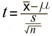
with the bottom portion referring to the estimated standard error. You may see this written as sM instead. Continue reading

Statistics: Introduction to Hypothesis Testing

Hypothesis Testing Basics

What is Hypothesis Testing?

Hypothesis testing is a big part of what we would actually consider testing for inferential statistics. It’s a procedure and set of rules that allow us to move from descriptive statistics to make inferences about a population based on sample data. It is a statistical method that uses sample data to evaluate a hypothesis about a population.

This type of test is usually used within the context of research. If we expect to see a difference between a treated and untreated group (in some cases the untreated group is the parameters we know about the population), we expect there to be a difference in the means between the two groups, but that the standard deviation remains the same, as if each individual score has had a value added or subtracted from it. Continue reading

Statistics: Distribution of Sample Means

Distribution of Sample Means

Up until this point, as far as distributions go, it’s been about being able to find individual scores on a distribution. Moving into hypothesis testing, we’re going to switch from working with very concrete distributions with scores to hypothetical distributions of sample means. In other words, we’re still working with normal distributions, but the points that make up the distribution will no longer be individual scores, but all possible sample means which can be drawn from a population with a given N or number of scores in them.

We use these kinds of distributions because with inferential statistics we’re going to want to find the probability of acquiring a certain sample mean to see if it’s common or very rare and therefore perhaps significantly different from another mean.

There are some concepts you will have to keep in mind for this shift including sampling error, the central limit theorem, and standard error. Continue reading

Statistics: Probability and Sampling

Introduction to Probability and Sampling

Probabilities

A probability is a fraction or a proportion of all the possible outcomes. So it’s the number of classified outcomes classified as X divided by the total number of possible outcomes (N). It’s generally reported as a decimal, but it can also be reported as a fraction or a percentage. 

What is the role of probability in populations, samples, and inferential statistics? As we discussed before, because it’s usually impossible for researchers to draw data from the entirety of a population, they draw samples. The size of the sample affects how comparable the sample population is to the general population. Probability is used to predict what kind of samples are likely to be obtained from a population. Thus, probability establishes a connection between samples and populations; we know from looking at the population how likely it is for a specific sample to be drawn. We also use proportions that exist within samples to infer the probabilities that exist within a population. Inferential statistics rely on this connection when they use sample data as the basis for making conclusions about populations. Continue reading

Statistics: Z-score Basics

Z-Score Introduction

Standardized Distributions

Sometimes when working with data sets, we want to have the scores on the distribution standardized. Essentially, this means that we convert scores from a distribution so that they fit into a model that can be used to compare and contrast distributions from different works. For example, if you have a distribution of scores that show the temperature each day over the summer in Boston, it may be recorded in Fahrenheit. Someone else in Paris may have recorded their summer temperatures as well but in Celcius. If we wanted to compare these distributions of scores based on their descriptive statistics, we may want to convert them to the same standardized unit of measurement. 

Standardized distributions have one single unit of measurement. Raw scores are transformed into this standardized unit of measurement to be compared to one another. Ultimately, they should look just like the original distribution, the only difference is that the scores have been placed on a different unit of measurement. Continue reading

Statistics: Variability

Basics of Variability

Variability is often a difficult topic for newcomers to statistics to grasp. Essentially it is the spread of the scores in a frequency distribution. If you have a bell curve which is pretty flat, you would say that it has high variability. If you have a bell curve which is pointy, you would say that it has low variability. Variability is really a quantitative measure of the differences between scores and describes the degree to which the score are spread out or clustered together. The purpose of measuring variability is to be able to describe the distribution and measure how well an individual score represents the distribution.

There are three main types of variability:

  • Range: The distance between the lowest and the highest score in a distribution. Can be described as one number or represented by writing out the lowest and highest number together (ex. values 4-10). Calculated by subtracting the highest score from the lowest score. If you’re working with continuous variables, it’s the upper real limit for Xmax minus the lower real limit for Xmin.
  • Standard deviation: The average distance between the scores in a data set and the mean. Here’s a video to help you conceptualize this. This value is also the square root of the variance.
  • Variance: Measures the average squared distance from the mean. This number is good for some calculations, but generally we want the standard deviation to determine how spread out a distribution is. Calculated with this equation:

Continue reading

Statistics: Measures of Central Tendency

Central Tendency

Central tendency is a statistical measure; a single score to define the center of a distribution. It is also used to find the single score that is most typical or best represents the entire group. No single measure is always best for both purposes. There are three main types:

  • Mean: sum of all scores divided by the number of scores in the data, also referred to as the average.
  • Median: the midpoint of the scores in a distribution when they are listen in order from smallest to largest. It divides the scores into two groups of equal size. With an even number of scores, you compute the average of the two middle scores.
  • Mode: the most frequently occurring number(s) in a data set.

Here are a variety of videos to help you understand the concepts of these measures, finding the median using a histogram, and finding a missing value given the mean. Continue reading