Monthly Archives: July 2019

Using SPSS: Comparing Means – Repeated Measures One-Way ANOVA

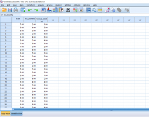
This post will be about finding a difference in means when it comes to repeated measures in research designs with a factor with more than 2 levels. Just like with the Repeated Measures t-test, we’ll be lining our levels up in columns. For this example, we’ll pretend that we’ve collected data on self-reported depression. Participants were asked to rate on a scale from 1-9 how severe they felt their depression is. They were then given medication to take which is known to reduce depressive symptoms. Participants were asked again after 6 months how high they rated their depression. They were asked one last time at the end of 12 months.

Continue reading

Using SPSS: Comparing Means – Repeated Measures t-test

In this section, we’ll be talking about how to properly conduct a repeated measures t-test on SPSS. Before, when we were working on independent t-tests, we needed to create a list of numbers which represented group categories so that the corresponding continuous data was grouped properly. In this kind of t-test though, each “Variable” actually becomes a level. In this case of this example, we’re looking at the data from a before and after. The “Before” consists of the number of alcoholic drinks 30 college students are consuming a week.  The “After” consists of the number of alcoholic drinks the same college students were drinking after having taken a Wellness class which focused on the effects of drug and alcohol on the mind and body. If you’re confused as to how this differs from an independent samples t-test, I suggest looking at the Independent Samples t-test and Repeated Measures t-test posts.  Continue reading

Statistics: Sampling Distribution of the Proportion

Sampling Distribution of the Proportion

In this section, we’ll be talking about finding the probability of a sample proportion. You may remember that a sampling distribution is a distribution not of scores, but all possible sample outcomes which can be drawn given that we’re working with a specific n. In this case, the following equations can help us figure out, based on a population proportion, how likely it is that we’ll draw a sample that has a chosen proportion. A question which would require these equations may sound like the following:

“A nation-wide survey was conducted about the perception of a brand. People were asked whether they liked the brand or disliked the brand and the results showed that 65% of people liked the brand. If we were to draw a random sample of 200 people, what is the probability that 80% of people within that sample will say they like the brand?”

The population proportion, denoted as ?, is the proportion of items in the entire population with the particular characteristic that we’re interested in investigating. The sample proportion, denoted by p, is the proportion of items in the sample with the characteristic that we’re interested in investigating. The sample proportion, which by definition is a statistic, is used to estimate the population proportion, which by definition is a parameter. Continue reading

Using SPSS: Comparing means – Independent Samples t-test

So far we’ve talked about creating independent variables, but what about levels? This may seem strange at first, but levels of a condition need to be spelled out by numbers. Usually, I just assign condition 1 a 1 and condition 2 a 2. You can see in the picture below how this looks. You can’t see this, but there are 30 individuals in total, half in condition 1, and half in condition 2.

Continue reading

Statistics: Discrete Probability Distributions

Introduction to Discrete Probability Distributions

Discrete versus Continuous Variables

A discrete variable typically originates from a counting process while a continuous variable usually comes from a measuring process. An easy way to make the distinction between a discrete and a continuous variable is that discrete variables are usually whole numbers with no decimals. Continuous variables on the other hand frequently take the form of decimals. For instance, the number of people which exist within a group is a discrete variable because it’s always a whole number, while a person’s weight would be continuous since it can typically be measured to multiple decimal places.

The Probability Distribution for a Discrete Variable

A probability distribution for a discrete variable is simply a compilation of all the range of possible outcomes and the probability associated with each possible outcome. Since, probability in general, by definition, must sum to 1, the summation of all the possible outcomes must sum to 1. For example, if you’re flipping a coin once, there’s a 1 in 2 chance it will land on heads, and a 1 in 2 chance it will land on tails; 1/2 + 1/2 = 1. In this way, measuring probability is similar to the use of percentages. Percentages are always measured out of 100 while probability is always measured out of 1. This is true for all probability measurements Continue reading

Using SPSS: Descriptive Statistics

Sometimes you’ll want to get some basic information on the data you have. Running these descriptive statistics is pretty straight forward. First, click the Analyze button, hover over the Descriptive Statistics tab, and then you’ll be able to choose a few different options. I prefer just clicking the frequencies button because it gives you the option to look at frequencies as well as other kinds of descriptives.

Continue reading