Tag Archives: #MATH115

Statistics: Reading Graphs for Two-Way ANOVAs

Reading graphs of two-way ANOVAs is often a little frustrating at first for students who are new to reading them. The goal of this post is to hopefully make the process more straight-forward.

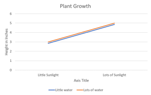
If you’re not sure already what a main effect or interaction is, I would suggest heading over to another post about two-way ANOVAs first. The purpose of one of these graphs is to help the reader visualize the results of the test when reading the results can sometimes be overwhelming, especially if the researchers are working with several different levels in each independent variable. The first trick to remember is that when looking for a significant main effect in the variable on the X-axis, we want the mean distance between the two points above one condition to be different from the mean distance between the two points of another condition. A clear example of this is below. The middle point between the orange line and blue line above “Little Sunlight” is around 2.8, while the middle point between the orange line and blue line above “Lots of Sunlight” is about 4.8. Given the context, we would say that there is a main effect for sunlight in which plant growth increases as levels of sunlight increase.

Continue reading

Using SPSS: Comparing Means – Independent Measures One-Way ANOVA

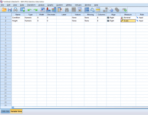
Just like an independent samples t-test, an Independent measures one-way ANOVA uses independent subjects for each level/condition within an independent variable. In this example, we’re growing plants. In Variable View, I’ve made the independent variable Condition (in this case the amount of water I’ll be giving to the plants) and the dependent variable Height.

Continue reading

Using SPSS: Comparing Means – Repeated Measures One-Way ANOVA

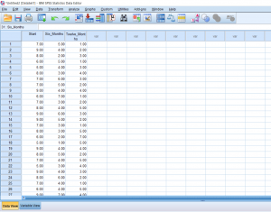
This post will be about finding a difference in means when it comes to repeated measures in research designs with a factor with more than 2 levels. Just like with the Repeated Measures t-test, we’ll be lining our levels up in columns. For this example, we’ll pretend that we’ve collected data on self-reported depression. Participants were asked to rate on a scale from 1-9 how severe they felt their depression is. They were then given medication to take which is known to reduce depressive symptoms. Participants were asked again after 6 months how high they rated their depression. They were asked one last time at the end of 12 months.

Continue reading

Using SPSS: Comparing Means – Repeated Measures t-test

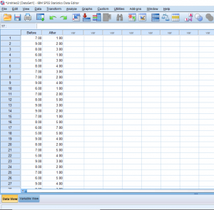
In this section, we’ll be talking about how to properly conduct a repeated measures t-test on SPSS. Before, when we were working on independent t-tests, we needed to create a list of numbers which represented group categories so that the corresponding continuous data was grouped properly. In this kind of t-test though, each “Variable” actually becomes a level. In this case of this example, we’re looking at the data from a before and after. The “Before” consists of the number of alcoholic drinks 30 college students are consuming a week.  The “After” consists of the number of alcoholic drinks the same college students were drinking after having taken a Wellness class which focused on the effects of drug and alcohol on the mind and body. If you’re confused as to how this differs from an independent samples t-test, I suggest looking at the Independent Samples t-test and Repeated Measures t-test posts.  Continue reading

Statistics: Choosing a Test

The following post is about breaking down the uses for different types of tests. More importantly, it’s designed to help you know what test to use based on the question being asked. This is not a comprehensive list of all the statistical tests out there, so if you feel that there is something missing which you would like to be included, please leave a comment below. All formulas for the tests presented here can be found in the Statistics Formula Glossary post. At the bottom is a decision tree which may be helpful in visualizing the purpose of this post. Continue reading

Statistics Formula Glossary

Stats Formula Glossary (Word) as of 7/16/2019

Stats Formula Glossary (PDF) as of 7/16/2019

Attached to this post are a PDF version and a Word document version of a glossary of formulas that may be helpful to keep around when practicing statistical problems for homework or studying for an upcoming test.

Please keep in mind that although these formulas work, they may not be the versions that your professors have taught you to use. It may also be that this formula sheet has formulas for problems you don’t need to know how to solve for the purposes of your class. If this is the case, we encourage you to download the Word document version so that you may add to, subtract from, or edit the glossary to fit your own individual needs.

Please keep in mind that this formula sheet may be edited after having been posted; the copy you download today may be different from the copy posted tomorrow. This list is by no means comprehensive of all formulas used in the field of statistics. If you have suggestions on formulas you would like to see added to this list, please leave a comment underneath of this post and we will take your suggestion into consideration. Good luck!

Statistics: Regression

Introduction to Linear Regression

Linear regression is a method for determining the best-fitting line through a set of data. In a lot of ways, it’s similar to a correlation since things like r and r squared are still used. The one difference is that the purpose of regression is prediction. The best-fitting line is calculated through the minimization of total squared error between the data points and the line.

The equation used for regression is Y = a +bx or some variation of that. If you remember from algebra class, this formula is like Y=mx+b. This is because they are both the linear equation. Although you may be asked to report r and r squared, the purpose of regression is to be able to find values for the slope (b) and the y-intercept (a) that creates a line that best fits through the data. Continue reading

Statistics: Correlation

Introduction to Correlation and Regression

So far we’ve been talking about analyses which involve variables which are split up into categorical or discrete variables (ex. treatment A, B, C) compared to a dependent variable which is continuous (ex. plant height). However, there is a way to look at two variables which have continuous data: correlation. A correlation will tell you the characteristics of a relationship such as direction (either positive or negative), form (we often work with linear relationships), and strength of the relationship. Strength and direction can be understood with the number which is given at the end of an analysis (r).

positive correlation is one in which the increased value of one variable results in the increased value of another. For example, height and weight – as height increased, weight also tends to increase. A negative correlation is one in which the increased value of one variable results in the decrease of another. For example, as the temperature outside increases, hot chocolate sales will decrease. This is what is meant by the direction of a correlation. An r-value with a negative sign in front of it means a negative correlation and one without a negative sign means a positive correlation. Continue reading

Statistics: Two-Factor ANOVA

Introduction to Two-Factor ANOVAs

So far we’ve talked about tests which are used if there is one independent variable, either with two levels or more. This is not the limit of how much we can include in a single analysis. In a two-factor ANOVA, there is more than one independent variable and each of those variables can have two or more levels. Take this example into consideration:

A farmer wants to know the best combination of products to use to maximize her crop yield. She decides to test out three different fertilizer brands (A, B, and C) and two different kinds of seeds (Y and Z). Each product is paired once with another for a total of 6 conditions: AY, BY, CY, AZ, BZ, CZ.

A two-factor ANOVA considers more than one factor and considers the joint impact of factors. This means that instead of running a new study every time you want to see how an independent variable affects a specific dependent variable, you can run an experiment with two different independent variables and seeing how they each impact the dependent variable and you get to see if the two independent variables do anything together to affect the dependent variable. These are called main effects and interactions. Keeping the example going, if we find that no matter what the seed type is that fertilizers A, B, and C resulted in different crop yields from one another, we would say there is a main effect for fertilizer type. If no matter what the fertilizer type is there is a difference between the crop yields of seeds Y and Z, we would say that there is a main effect for seed type. If there are times that the two factors influence each other (for example, let’s say that fertilizer worked much better specifically when paired with Y seeds), we would say there’s an interaction.  The defining characteristic of an interaction is when the effect of one factor depends on the different levels of a second factor or the impact of another factor, either amplifying or reducing the effect based on the level. Continue reading

Statistics: Repeated Measures ANOVA

Repeated Measures One-way ANOVA

Just like when we talked about independent samples t-tests and repeated measures t-tests, ANOVAs can have the same distinction. Independent one-way ANOVAs use samples which are in no way related to each other; each sample is completely random, uses different individuals, and those individuals are not paired in any meaningful way. In a repeated measures one-way ANOVA, individuals can be in multiple treatment conditions, be paired with other individuals based on important characteristics, or simply matched based on a relationship to one another (twins, siblings, couples, etc.). What’s important to remember that in a repeated measures one-way ANOVA, we are still given the opportunity to work with multiple levels, not just two like with a t-test.

Advantages:

  • Individual differences among participants do not influence outcomes or influence them very little because everyone is either paired up on important participant characteristics or they are the same person in multiple conditions.
  • A smaller number of subjects needed to test all the treatments.
  • Ability to assess an effect over time.

Continue reading